Last month, I finished going through Nathan Braun’s Coding with Baseball, a book I purchased around four years ago. If you’re at all interested in baseball statistics and want to build a quick foundation for exploring them, I highly recommend the book. It doesn’t hold your hand—it’s not a reference text, and you’ll need documentation for pandas, seaborn, and scikitlearn for the exercises—but it’s an excellent, concise overview that teaches exactly what you need with a straightforward style and relevant examples. It encouraged me to set up the Lahman Baseball Database on my computer and led me down a few rabbit holes, one of which I’ll explain here.
Random Forest Regression
Chapter 7 discusses statistical modeling.1 I was fascinated by the Random Forest methods—they were entirely new to me, and it amazed me how quick it was to put together. That being said, the example provided in the books is specifically a Random Forest model for categorical data—in this case, pitch type. Then there’s this throwaway line that got me interested.
If you’re modeling a continuous valued variable (like on base percentage or number of hits in a season) you do the exact same thing, but with
RandomForestRegressorinstead.
There are no exercises to conclude this chapter, so this was a clear option. An awesome feature of the RandomForestClassifier model is its inbuilt confidence metrics. I wanted to build a model for pitch velocity based on the many available factors I had—pitch location, spin rate and direction, game situation—and understand the confidence of each prediction and the model as a whole. However, the Regressor model has no analogous confidence metric, so I turned to Claude for some help.
After some back-and-forth while I interrogated their suggestions, we initially landed on the confidence score metric 1/(1 + std), where std is the standard deviation across the component Random Forest predictions. The more varied the predictions are, the less confident the model is. However, I pointed out that this is not a linear confidence score, so it’s hard to make sense of it. One quick change later—obtaining percentile ranks via the .rank(pct=True) method on a series—got me there.
Here’s the final table of confidence scores grouped by pitch type.
| CH (Changeup) | 0.246479 |
|---|---|
| CU (Curve ball) | 0.517901 |
| EP (Eephus) | 0.143597 |
| FC (Cutter) | 0.554579 |
| FF (4-seam Fastball) | 0.603719 |
| FS (Splitter) | 0.432211 |
| FT (2-seam Fastball) | 0.404022 |
| KC (Knuckle Curve) | 0.524997 |
| SI (Sinker) | 0.411485 |
| SL (Slider) | 0.511924 |
Gradient Boost
Since I was already talking with Claude, asking what other tools may be appropriate for this analysis made sense. It gave me three options, and I decided to go for Gradient Boost. This is where I can give LLMs their due—this was a fascinating and fruitful conversation that still relied on me paying attention. You can follow the link above to see the full conversation, but here are some highlights that resulted in great responses.
(MR) Yes, let’s try your Gradient Boosting idea. In addition to the code, could you please give me a brief overview of how this method works under the hood? You don’t need to get too technical—a metaphorical explanation is great if you have one.
(Claude) Let me give you an analogy for Gradient Boosting first: Imagine you’re trying to guess someone’s weight by looking at their height, age, and build. Your first guess might be based just on height and be pretty rough. Then, instead of starting over, you look at where you made mistakes and make small corrections based on age. Then you look at where you’re still making mistakes and make additional small corrections based on build. Each time, you’re focusing on fixing the errors from your previous guesses.
That’s essentially what Gradient Boosting does - it builds a sequence of simple models (usually decision trees), where each new model tries to correct the mistakes of the combined previous models.
I asked one follow-up question about the model parameters, but the code Claude provided after its metaphorical explanation worked on the first try. I noticed something odd about the confidence scores between Random Forest and Gradient Boost given how the models performed and asked Claude about it:
(MR) I’m now more interested in comparing the results from the Random Tree and the Gradient Boost models. At least when comparing the final results, their mean average errors are quite similar, with Gradient Boost being about 8% larger error. However, the standard deviations for Gradient Boost are an order of magnitude larger, and all of the confidence scores are extremely low. This is surprising given the final results are so close. Is it fair to assume this massive difference in the “component model results” is because Gradient Boost is always starting from a worst initial model that it’s refining, while Random Tree is building many distinct, but similarly competent, models along the way?
Claude confirmed my suspicions and, after I asked, suggested we only consider the final 20% of stages in each Gradient Boost model for the sake of computing confidence. It then suggested the following code to create a single dataframe that could provide confidence comparisons by pitch type.
comparison = test.groupby('pitch_type').agg({
    'mph_confidence_percentile': 'mean',  # RF confidence
    'mph_confidence_percentile_xgb_v2': 'mean'  # XGB confidence
}).round(3)
Once again, it was vital that I actively participated in this conversation and had my own thoughts about what I was trying to accomplish. Taking a straight mean doesn’t quite make sense here because the number of observations is highly variable between pitch types. A weighted average/expected value makes more sense when directly comparing them. So, I added these.
comparison['exp_cp'] = comparison['mph_cp'] * comparison['num_pitches']
comparison['exp_cp_xgb'] = comparison['mph_cp_xgb'] * comparison['num_pitches']

comparison['exp_cp'].sum()
comparison['exp_cp_xgb'].sum()
The final results gave the Random Forest model a weighted confidence score of 2945.7, and the Gradient Boost model a score of 2944.0.
Pretty Pictures
I was a bit out of my depth when trying to plot the original Random Forest model for pitch velocity along with its confidence score. I know I wanted to use seaborn—the tool of choice in Chapter 6 on data visualization—but I started broadly.
(MR) Let’s shift to visualizing this data. What are some interesting ways to visualize the output of these models, include their confidence in some way?
We’d only been working in Python, so I assumed I’d get a solution that way. Instead, Claude fed me some Javascript React code. I suggested we use seaborn and matplotlib, and it corrected itself with some mostly working code. As it happens, seaborn very recently made some changes to its set of “style” options, so I had to explore the documentation, but that was a quick fix.
With that out of the way, I was able to make some killer figures. There was a bit of iteration where labels showed up in odd places, but we sorted it out. I leave the figures below to observe without comment.
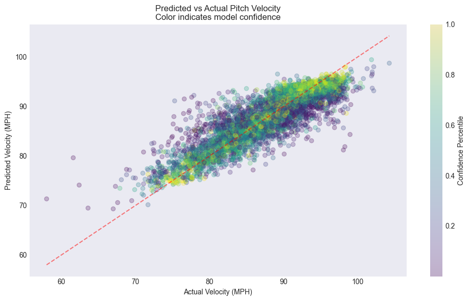
All observations
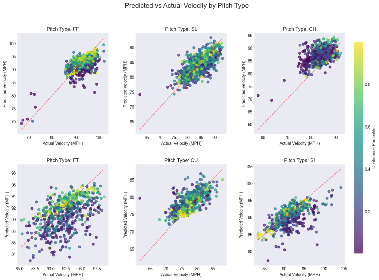
Broken out by pitch type.
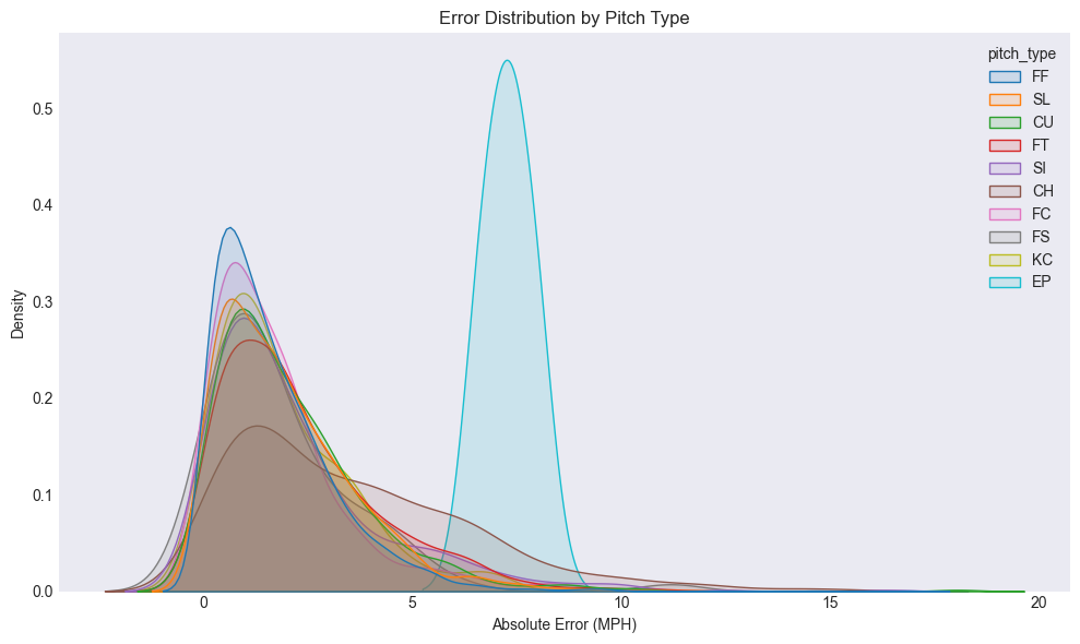
There are only 1 or 2 eephus pitches, so that distribution stands out.
I’m the least impressed by this chapter, but the book’s author is clearly unconcerned with statistical and mathematical rigor. This is a rough introduction, and I accept it for what it is. ↩︎